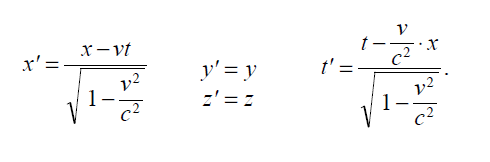
Lorentz transformation looks at the characteristics of space and time from the viewpoint of the invariant speed of light. The invariance of the speed of light means that it is absolute. It does not depend on anything external to light. It is an intrinsic property.
.
Light as Substance
If light has
intrinsic properties, then light may be considered a substance. Newton thought
so because he looked at light as made up of corpuscles. Unlike an atom a
corpuscle is infinitely divisible. See Corpuscular theory of
light – Wikipedia. An
“electromagnetic cycle” may be considered a corpuscle. It is infinitely divisible
because time can be considered to be infinitely divisible.
The higher is
the frequency of light, the greater is the concentration of “electromagnetic
cycles”, or corpuscles. These corpuscles cannot be treated as point particles
because they do not have center of mass like material particles do. They have
to treated as a fluid-like continuum. Therefore, higher concentration of
corpuscles would mean, higher density of the fluid-like continuum of light.
We may conclude that light is a continuum with certain density. Its density is represented by a “frequency”. This density indicates that light has mass, but this mass is not structured as it is in matter. This mass displays wave characteristics as it flows at the speed of light.
.
Space and Time
Space may be
considered to be a characteristic of substance. Descartes thought that space is
defined by the extents of substance. This is obvious for matter. But the space,
which is empty of matter, may actually be defined by the extents of light. Here
light refers to the whole electromagnetic spectrum.
Similarly, time may be defined by the duration of substance. Matter seems to have almost infinite duration because it endures forever at any location in space. But the duration of light seems to be very small, because it whizzes past any location in space at great speed. The duration of a substance and its absolute speed appear to be inverse of each other. See The Logic of Motion.
.
Speed in Lorentz Equation
The above considerations present motion in absolute terms. They are
very likely to provide interesting interpretation to Lorentz transformations
and also to Einstein’s theory of special relativity.
The relative motion that we measure as the speed of heavenly bodies and the speed of objects on earth, is not the same thing as the absolute motion that we measure as inverse of density. Therefore, we cannot compare a relative speed to the absolute motion of light because they do not have the same basis. They are like apples and oranges. The “v/c” ratio in Lorentz transform have no consistent basis mathematically.
The implications of this shall be taken up in the next chapter.
I asked this question on Quora: If photon is massless, how is mass defined in physics? Most answers that I got were cookie cutter answers from quantum mechanics perspective that do not see the following inconsistencies:
(1) The concept of particle comes from matter. A material particle is discrete because it can be treated mathematically as a point particle as it has a center of mass. The concept of particle ends when there is no center of mass.
(2) Electrons have mass, but no center of mass. In the absence of center of mass a particle cannot be distinguished from another particle. There is still mass but no discreteness. Electrons are, therefore, a fluid-like continuum rather than discrete particle-like collection. This logic is ignored by quantum mechanics.
(3) Energy interactions are always discrete because it takes a precise amount of energy for a unique interaction to take place. But a discrete energy interaction does not imply that the interacting elements are discrete in space also. Einstein’s “energy particle” is a discrete energy interaction. It was an error to assume that a discrete “energy particle” is also a discrete “mass particle” in space.
Electrons and light are fluid-like continuum per the above logic, but they can have discrete energy interactions. That is perfectly okay. Electrons and light are fluid like continuum is confirmed by the mathematics of Quantum Electrodynamic, as shown by Richard Feynman in his lecture on quantum behavior. Please see Feynman on Quantum Behavior.
What is missed by quantum mechanics is that mass can be fluid-like continuum that is infinitely divisible. This is what Newton implied in his Corpuscular theory of Light. From Corpuscular theory of light – Wikipedia:
“Corpuscular theories… are similar to the theories of atomism, except that in atomism the atoms were supposed to be indivisible, whereas corpuscles could in principle be divided. Corpuscles are single, infinitesimally small, particles which have shape, size, color, and other physical properties which alter their functions and effects in phenomena in the mechanical and biological sciences.”
Corpuscles, thus, provide a dimension of fluid-like continuum of “mass concentrations” that can be reduced indefinitely. These concentrations are represented by the frequency of EMR. Frequencies formed the basis of the original concept of quantum.
The idea of “rest mass” may be understood as follows: If we are traveling at the speed of light along side a beam of light, that beam shall appear as a fluid continuum that has the mass concentration of E/c^2. Mass is more basic than energy. Kinetic energy is the energy of moving mass.
Light’s speed is intrinsic and finite because of its mass concentration. Please see The Logic of Motion.
.
Addition Nov 9, 2022:
Originally, a particle was understood to be a small part of matter that obviously had a fied boundary and a center of mass. Example of this would be a dust particle, or a particle of sand. In Chemistry, a particle was related to parts of substance that took part in a chemical reaction. Ultimately, a particle of matter was reduced to the idea of an atom or a molecule. Its boundaries were considered to be well defined and fixed, and it had a center of mass.
This idea of particle shifted as one looked at the sub-atomic region beyond the nucleus. Here the substance is no longer rigidly structured as in the case of matter, or even an atom. This sub-atomic substance is rather thin in consistency and spread out. It appears as a continuum with no definite boundaries and no center of mass. Only definite amount of this subtance seem to take part in sub-atomic reactions. Therefore, we fall back on concept of particle similar to that in Chemistry. It is a definite amount of “energy substance” that takes part in a reaction. At sub-atomic level, this is referred to as a “quantum.”
Therefore, in its most basic sense, a particle is defined in terms of its associations. And that, by definition, is a perceptual element.
The original material is in black, main points are in brown, and the comments are noted in blue based on present understanding. The heading below is linked to the original materials.
NOTE: Light is a continuum of substance that is infinitely divisible. A photon is a discrete amount drawn from this continuum for interaction (see Particle, Continuum and Atom). Feynman’s mathematics actually treats light as a continuum as it should.
“Quantum mechanics” is the description of the
behavior of matter and light in all its details and, in particular, of the
happenings on an atomic scale. Things on a very small scale behave like nothing
that you have any direct experience about. They do not behave like waves, they
do not behave like particles, they do not behave like clouds, or billiard balls,
or weights on springs, or like anything that you have ever seen.
Things on a very small scale behave very differently.
Newton thought that light was made up of particles, but then it was discovered that it behaves like a wave. Later, however (in the beginning of the twentieth century), it was found that light did indeed sometimes behave like a particle. Historically, the electron, for example, was thought to behave like a particle, and then it was found that in many respects it behaved like a wave. So it really behaves like neither. Now we have given up. We say: “It is like neither.”
NOTE: Light is a continuum of substance that has very small density. The infinite divisibility of light as a continuum gives it wave characteristics. The density of light allows it to make impact. Light is neither a particle nor a wave disturbance.
There is
one lucky break, however—electrons behave just like light. The quantum behavior
of atomic objects (electrons, protons, neutrons, photons, and so on) is the
same for all, they are all “particle waves,” or whatever you want to call them.
So what we learn about the properties of electrons (which we shall use for our
examples) will apply also to all “particles,” including photons of light.
NOTE: Electrons are also a continuum, but they are much denser than light. All quantum “particles” are continua. They are “particles” only in the sense of energy interactions.
The gradual accumulation of information about atomic and small-scale behavior during the first quarter of the 20th century, which gave some indications about how small things do behave, produced an increasing confusion which was finally resolved in 1926 and 1927 by Schrödinger, Heisenberg, and Born. They finally obtained a consistent description of the behavior of matter on a small scale. We take up the main features of that description in this chapter.
The behavior of substances at atomic scale was finally settled around 1926-27.
Because
atomic behavior is so unlike ordinary experience, it is very difficult to get
used to, and it appears peculiar and mysterious to everyone—both to the novice
and to the experienced physicist. Even the experts do not understand it the way
they would like to, and it is perfectly reasonable that they should not,
because all of direct, human experience and of human intuition applies to large
objects. We know how large objects will act, but things on a small scale just
do not act that way. So we have to learn about them in a sort of abstract or
imaginative fashion and not by connection with our direct experience.
NOTE: Larger objects behave like particles, but things on small scale behave like continua.
In this chapter we shall tackle immediately the basic element of the mysterious behavior in its most strange form. We choose to examine a phenomenon which is impossible, absolutely impossible, to explain in any classical way, and which has in it the heart of quantum mechanics. In reality, it contains the only mystery. We cannot make the mystery go away by “explaining” how it works. We will just tell you how it works. In telling you how it works we will have told you about the basic peculiarities of all quantum mechanics.
NOTE: We need to understand how continua behave as opposed to particles.
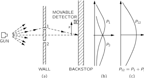
1–2 An experiment with bullets
Fig. 1–1. Interference experiment with bullets.
To try to understand the quantum behavior of electrons, we shall compare and contrast their behavior, in a particular experimental setup, with the more familiar behavior of particles like bullets, and with the behavior of waves like water waves. We consider first the behavior of bullets in the experimental setup shown diagrammatically in Fig. 1–1. We have a machine gun that shoots a stream of bullets. It is not a very good gun, in that it sprays the bullets (randomly) over a fairly large angular spread, as indicated in the figure. In front of the gun we have a wall (made of armor plate) that has in it two holes just about big enough to let a bullet through. Beyond the wall is a backstop (say a thick wall of wood) which will “absorb” the bullets when they hit it. In front of the backstop we have an object which we shall call a “detector” of bullets. It might be a box containing sand. Any bullet that enters the detector will be stopped and accumulated. When we wish, we can empty the box and count the number of bullets that have been caught. The detector can be moved back and forth (in what we will call the x-direction). With this apparatus, we can find out experimentally the answer to the question: “What is the probability that a bullet which passes through the holes in the wall will arrive at the backstop at the distance x from the center?” First, you should realize that we should talk about probability, because we cannot say definitely where any particular bullet will go. A bullet which happens to hit one of the holes may bounce off the edges of the hole, and may end up anywhere at all. By “probability” we mean the chance that the bullet will arrive at the detector, which we can measure by counting the number which arrive at the detector in a certain time and then taking the ratio of this number to the total number that hit the backstop during that time. Or, if we assume that the gun always shoots at the same rate during the measurements, the probability we want is just proportional to the number that reach the detector in some standard time interval.
For our present purposes we would like to imagine a somewhat idealized experiment in which the bullets are not real bullets, but are indestructible bullets—they cannot break in half. In our experiment we find that bullets always arrive in lumps, and when we find something in the detector, it is always one whole bullet. If the rate at which the machine gun fires is made very low, we find that at any given moment either nothing arrives, or one and only one—exactly one—bullet arrives at the backstop. Also, the size of the lump certainly does not depend on the rate of firing of the gun. We shall say: “Bullets always arrive in identical lumps.” What we measure with our detector is the probability of arrival of a lump. And we measure the probability as a function of x. The result of such measurements with this apparatus (we have not yet done the experiment, so we are really imagining the result) are plotted in the graph drawn in part (c) of Fig. 1–1. In the graph we plot the probability to the right and x vertically, so that the x-scale fits the diagram of the apparatus. We call the probability P12 because the bullets may have come either through hole 1 or through hole 2. You will not be surprised that P12 is large near the middle of the graph but gets small if x is very large. You may wonder, however, why P12 has its maximum value at x=0. We can understand this fact if we do our experiment again after covering up hole 2, and once more while covering up hole 1. When hole 2 is covered, bullets can pass only through hole 1, and we get the curve marked P1 in part (b) of the figure. As you would expect, the maximum of P1 occurs at the value of x which is on a straight line with the gun and hole 1. When hole 1 is closed, we get the symmetric curve P2 drawn in the figure. P2 is the probability distribution for bullets that pass through hole 2. Comparing parts (b) and (c) of Fig. 1–1, we find the important result that
P12 = P1 + P2. (1.1)
The probabilities
just add together. The effect with both holes open is the sum of the effects
with each hole open alone. We shall call this result an observation of “no interference,” for a reason that you will see later.
So much for bullets. They come in lumps, and their probability of arrival shows
no interference.
NOTE: The hole is slightly bigger than the bullet to let it through. The bullets cannot be split into parts. They act like an indivisible particles. There aren’t many ways in which the two streams of bullets emerging from the slit can interfere with each other.So the outcome is a summation as shown.
1–3 An experiment with waves
Fig. 1–2. Interference experiment with water waves.
Now we wish to consider an experiment with water waves. The apparatus is shown diagrammatically in Fig. 1–2. We have a shallow trough of water. A small object labeled the “wave source” is jiggled up and down by a motor and makes circular waves. To the right of the source we have again a wall with two holes, and beyond that is a second wall, which, to keep things simple, is an “absorber,” so that there is no reflection of the waves that arrive there. This can be done by building a gradual sand “beach.” In front of the beach we place a detector which can be moved back and forth in the x-direction, as before. The detector is now a device which measures the “intensity” of the wave motion. You can imagine a gadget which measures the height of the wave motion, but whose scale is calibrated in proportion to the square of the actual height, so that the reading is proportional to the intensity of the wave. Our detector reads, then, in proportion to the energy being carried by the wave—or rather, the rate at which energy is carried to the detector.
With our
wave apparatus, the first thing to notice is that the intensity can have any size. If the source just moves a very small
amount, then there is just a little bit of wave motion at the detector. When
there is more motion at the source, there is more intensity at the detector.
The intensity of the wave can have any value at all. We would not say that there was any “lumpiness” in the wave
intensity.
Now let us measure the wave intensity for various values of x (keeping the wave source operating always in the same way). We get the interesting-looking curve marked I12 in part (c) of the figure.
We have already worked out how such patterns can come about when we studied the interference of electric waves in Volume I. In this case we would observe that the original wave is diffracted at the holes, and new circular waves spread out from each hole. If we cover one hole at a time and measure the intensity distribution at the absorber we find the rather simple intensity curves shown in part (b) of the figure. I1 is the intensity of the wave from hole 1 (which we find by measuring when hole 2 is blocked off) and I2 is the intensity of the wave from hole 2 (seen when hole 1 is blocked).
The intensity I12 observed when both holes are open is certainly not the sum of I1 and I2. We say that there is “interference” of the two waves. At some places (where the curve I12 has its maxima) the waves are “in phase” and the wave peaks add together to give a large amplitude and, therefore, a large intensity. We say that the two waves are “interfering constructively” at such places. There will be such constructive interference wherever the distance from the detector to one hole is a whole number of wavelengths larger (or shorter) than the distance from the detector to the other hole.
At those places where the two waves arrive at the detector with a phase difference of π (where they are “out of phase”) the resulting wave motion at the detector will be the difference of the two amplitudes. The waves “interfere destructively,” and we get a low value for the wave intensity. We expect such low values wherever the distance between hole 1 and the detector is different from the distance between hole 2 and the detector by an odd number of half-wavelengths. The low values of I12 in Fig. 1–2 correspond to the places where the two waves interfere destructively.
You will remember that the quantitative relationship between I1, I2, and I12 can be expressed in the following way: The instantaneous height of the water wave at the detector for the wave from hole 1 can be written as (the real part of) h1eiωt, where the “amplitude” h1 is, in general, a complex number. The intensity is proportional to the mean squared height or, when we use the complex numbers, to the absolute value squared |h1|2. Similarly, for hole 2 the height is h2eiωt and the intensity is proportional to |h2|2. When both holes are open, the wave heights add to give the height (h1 + h2)eiωt and the intensity |h1 + h2|2. Omitting the constant of proportionality for our present purposes, the proper relations for interfering waves are
I1=|h1|2, I2=|h2|2, I12=|h1 + h2|2. (1.2)
You will notice that the result is quite different from that obtained with bullets (Eq. 1.1). If we expand |h1 + h2|2 we see that
|h1 + h2|2 = |h1|2 + |h2|2 + 2|h1||h2|cosδ, (1.3)
where δ is the phase difference between h1 and h2. In terms of the intensities, we could write
I12 = I1 + I2 + 2√(I1I2) cos δ. (1.4)
The last term in (1.4) is the “interference term.” So much for water waves. The intensity can have any value, and it shows interference.
The waves divide at the holes. The two waves then combine in their amplitudes constructively and destructively as they overlap each other. The bullets do not show this behavior.
NOTE: In this case the wave disturbance is infinitely divisible. It can be split between the two holes in infinitely different ways. This makes all the difference in terms of getting an interference pattern.
1–4 An experiment with electrons
Fig. 1–3. Interference experiment with electrons.
Now we imagine a similar experiment with electrons. It is shown diagrammatically in Fig. 1–3. We make an electron gun which consists of a tungsten wire heated by an electric current and surrounded by a metal box with a hole in it. If the wire is at a negative voltage with respect to the box, electrons emitted by the wire will be accelerated toward the walls and some will pass through the hole. All the electrons which come out of the gun will have (nearly) the same energy. In front of the gun is again a wall (just a thin metal plate) with two holes in it. Beyond the wall is another plate which will serve as a “backstop.” In front of the backstop we place a movable detector. The detector might be a Geiger counter or, perhaps better, an electron multiplier, which is connected to a loudspeaker.
We should
say right away that you should not try to set up this experiment (as you could
have done with the two we have already described). This experiment has never
been done in just this way. The trouble is that the apparatus would have to be
made on an impossibly small scale to show the effects we are interested in. We
are doing a “thought experiment,” which we have chosen because it is easy to
think about. We know the results that would be obtained
because there are many experiments that have
been done, in which the scale and the proportions have been chosen to show the
effects we shall describe.
The first thing we notice with our electron experiment is that we hear sharp “clicks” from the detector (that is, from the loudspeaker). And all “clicks” are the same. There are no “half-clicks.”
We would also notice that the “clicks” come very erratically. Something like: click ….. click-click … click …….. click …. click-click …… click …, etc., just as you have, no doubt, heard a geiger counter operating. If we count the clicks which arrive in a sufficiently long time—say for many minutes—and then count again for another equal period, we find that the two numbers are very nearly the same. So we can speak of the average rate at which the clicks are heard (so-and-so-many clicks per minute on the average).
As we
move the detector around, the rate at which
the clicks appear is faster or slower, but the size (loudness) of each click is
always the same. If we lower the temperature of the wire in the gun, the rate
of clicking slows down, but still each click sounds the same. We would notice
also that if we put two separate detectors at the backstop, one or the other would click, but never both at once.
(Except that once in a while, if there were two clicks very close together in
time, our ear might not sense the separation.) We conclude, therefore, that
whatever arrives at the backstop arrives in “lumps.” All the “lumps” are the
same size: only whole “lumps” arrive, and they arrive one at a time at the
backstop. We shall say: “Electrons always arrive in identical lumps.”
NOTE: A click is generated when a certain amount of electron accumulates at the detector. We are simply detecting an energy particle. It does not imply that electrons exist in space as lumps. Electron actually exist as a continuum because they do not have center of mass.
Just as
for our experiment with bullets, we can now proceed to find experimentally the
answer to the question: “What is the relative probability that an electron
‘lump’ will arrive at the backstop at various distances x from the center?” As
before, we obtain the relative probability by observing the rate of clicks,
holding the operation of the gun constant. The probability that lumps will
arrive at a particular x is proportional to the average rate of
clicks at that x.
The result of our experiment is the interesting curve marked P12 in part (c) of Fig. 1–3. Yes! That is the way electrons go.
Electrons show interference patterns that is the characteristic of wave-like motion.
NOTE: This confirms that electron is a continuum that is infinitely divisible in space.
1–5 The interference of electron waves
Now let us try to analyze the curve of Fig. 1–3 to see whether we can understand the behavior of the electrons. The first thing we would say is that since they come in lumps, each lump, which we may as well call an electron, has come either through hole 1 or through hole 2. Let us write this in the form of a “Proposition”:
Proposition A: Each electron either goes through
hole 1 or it
goes through hole 2.
NOTE: Electrons are an infinitely divisible continuum in space and the proposition above is not correct.
Assuming Proposition A, all electrons that arrive at the backstop can be divided into two classes: (1) those that come through hole 1, and (2) those that come through hole 2. So our observed curve must be the sum of the effects of the electrons which come through hole 1 and the electrons which come through hole 2. Let us check this idea by experiment. First, we will make a measurement for those electrons that come through hole 1. We block off hole 2 and make our counts of the clicks from the detector. From the clicking rate, we get P1. The result of the measurement is shown by the curve marked P1 in part (b) of Fig. 1–3. The result seems quite reasonable. In a similar way, we measure P2, the probability distribution for the electrons that come through hole 2. The result of this measurement is also drawn in the figure.
The result P12 obtained with both holes open is clearly not the sum of P1 and P2, the probabilities for each hole alone. In analogy with our water-wave experiment, we say: “There is interference.”
For electrons: P12 ≠ P1 + P2. (1.5)
How can such an interference come about? Perhaps we should say: “Well, that means, presumably, that it is not true that the lumps go either through hole 1 or hole 2, because if they did, the probabilities should add. Perhaps they go in a more complicated way. They split in half and …” But no! They cannot, they always arrive in lumps … “Well, perhaps some of them go through 1, and then they go around through 2, and then around a few more times, or by some other complicated path … then by closing hole 2, we changed the chance that an electron that started out through hole 1 would finally get to the backstop …” But notice! There are some points at which very few electrons arrive when both holes are open, but which receive many electrons if we close one hole, so closing one hole increased the number from the other. Notice, however, that at the center of the pattern, P12 is more than twice as large as P1 + P2. It is as though closing one hole decreased the number of electrons which come through the other hole. It seems hard to explain both effects by proposing that the electrons travel in complicated paths.
It is all quite mysterious. And the more you look at it the more mysterious it seems. Many ideas have been concocted to try to explain the curve for P12 in terms of individual electrons going around in complicated ways through the holes. None of them has succeeded. None of them can get the right curve for P12 in terms of P1 and P2.
Yet, surprisingly enough, the mathematics for relating P1 and P2 to P12 is extremely simple. For P12 is just like the curve I12 of Fig. 1–2, and that was simple. What is going on at the backstop can be described by two complex numbers that we can call ϕ1 and ϕ2 (they are functions of x, of course). The absolute square of ϕ1 gives the effect with only hole 1 open. That is, P1= |ϕ1|2. The effect with only hole 2 open is given by ϕ2 in the same way. That is, P2=|ϕ2|2. And the combined effect of the two holes is just P12=|ϕ1 + ϕ2|2. The mathematics is the same as that we had for the water waves! (It is hard to see how one could get such a simple result from a complicated game of electrons going back and forth through the plate on some strange trajectory.)
We
conclude the following: The electrons arrive in lumps, like particles, and the
probability of arrival of these lumps is distributed like the distribution of
intensity of a wave. It is in this sense that an electron behaves “sometimes
like a particle and sometimes like a wave.”
Incidentally,
when we were dealing with classical waves we defined the intensity as the mean
over time of the square of the wave amplitude, and we used complex numbers as a
mathematical trick to simplify the analysis. But in quantum mechanics it turns
out that the amplitudes must be
represented by complex numbers. The real parts alone will not do. That is a
technical point, for the moment, because the formulas look just the same.
Since the probability of arrival through both holes is given so simply, although it is not equal to (P1 + P2), that is really all there is to say. But there are a large number of subtleties involved in the fact that nature does work this way. We would like to illustrate some of these subtleties for you now. First, since the number that arrives at a particular point is not equal to the number that arrives through 1 plus the number that arrives through 2, as we would have concluded from Proposition A, undoubtedly we should conclude that Proposition A is false. It is not true that the electrons go either through hole 1 or hole 2. But that conclusion can be tested by another experiment.
The assumption made in the Proposition A must be checked.
NOTE: The mathematics is the same as that we had for the water waves because in both cases we have a continuum that is infinitely divisible. In this case we are measuring quanta from kinetic energy of electron flow and not the intensity of wave disturbance.
1–6 Watching the electrons
Fig. 1–4. A different electron experiment.
We shall now try the following experiment. To our electron apparatus we add a very strong light source, placed behind the wall and between the two holes, as shown in Fig. 1–4. We know that electric charges scatter light. So when an electron passes, however it does pass, on its way to the detector, it will scatter some light to our eye, and we can see where the electron goes. If, for instance, an electron were to take the path via hole 2 that is sketched in Fig. 1–4, we should see a flash of light coming from the vicinity of the place marked A in the figure. If an electron passes through hole 1, we would expect to see a flash from the vicinity of the upper hole. If it should happen that we get light from both places at the same time, because the electron divides in half … Let us just do the experiment!
Here is
what we see: every time that we hear a
“click” from our electron detector (at the backstop), we also see a flash of light either near hole 1 or near hole 2, but never both at
once! And we observe the same result no matter where we put the detector. From
this observation we conclude that when we look at the electrons we find that
the electrons go either through one hole or the other. Experimentally,
Proposition A is necessarily true.
NOTE: When we put another detector near the holes we are looking at another energy interaction that is similar to the interaction at the detector at the wall. Discrete energy interactions do not necessarily imply spatial discreteness. Therefore, this does not confirm Proposition A.
What, then, is wrong with our argument against Proposition A? Why isn’t P12 just equal to P1 + P2? Back to experiment! Let us keep track of the electrons and find out what they are doing. For each position (x-location) of the detector we will count the electrons that arrive and also keep track of which hole they went through, by watching for the flashes. We can keep track of things this way: whenever we hear a “click” we will put a count in Column 1 if we see the flash near hole 1, and if we see the flash near hole 2, we will record a count in Column 2. Every electron which arrives is recorded in one of two classes: those which come through 1 and those which come through 2. From the number recorded in Column 1 we get the probability P’1that an electron will arrive at the detector via hole 1; and from the number recorded in Column 2 we get P’2, the probability that an electron will arrive at the detector via hole 2. If we now repeat such a measurement for many values of x, we get the curves for P’1 and P’2 shown in part (b) of Fig. 1–4.
Well, that is not too surprising! We get for P’1 something quite similar to what we got before for P1 by blocking off hole 2; and P’2 is similar to what we got by blocking hole 1. So there is not any complicated business like going through both holes. When we watch them, the electrons come through just as we would expect them to come through. Whether the holes are closed or open, those which we see come through hole 1 are distributed in the same way whether hole 2 is open or closed.
But wait! What do we have now for the total probability, the probability that an electron will arrive at the detector by any route? We already have that information. We just pretend that we never looked at the light flashes, and we lump together the detector clicks which we have separated into the two columns. We must just add the numbers. For the probability that an electron will arrive at the backstop by passing through either hole, we do find P’12 = P’1 + P’2. That is, although we succeeded in watching which hole our electrons come through, we no longer get the old interference curve P12, but a new one, P’12, showing no interference! If we turn out the light P12 is restored.
We must conclude that when we look at the electrons the distribution of them on the screen is different than when we do not look. Perhaps it is turning on our light source that disturbs things? It must be that the electrons are very delicate, and the light, when it scatters off the electrons, gives them a jolt that changes their motion. We know that the electric field of the light acting on a charge will exert a force on it. So perhaps we should expect the motion to be changed. Anyway, the light exerts a big influence on the electrons. By trying to “watch” the electrons we have changed their motions. That is, the jolt given to the electron when the photon is scattered by it is such as to change the electron’s motion enough so that if it might have gone to where P12 was at a maximum it will instead land where P12 was a minimum; that is why we no longer see the wavy interference effects.
You may
be thinking: “Don’t use such a bright source! Turn the brightness down! The light
waves will then be weaker and will not disturb the electrons so much. Surely,
by making the light dimmer and dimmer, eventually the wave will be weak enough
that it will have a negligible effect.” O.K. Let’s try it. The first thing we
observe is that the flashes of light scattered from the electrons as they pass
by does not get weaker. It is always the same-sized
flash. The only thing that happens as the light is made dimmer is
that sometimes we hear a “click” from the detector but see no flash at all. The electron has gone by without being
“seen.” What we are observing is that light also acts like
electrons, we knew that it was “wavy,” but
now we find that it is also “lumpy.” It always arrives—or is scattered—in lumps
that we call “photons.” As we turn down the intensity of
the light source we do not change the size of the
photons, only the rate at which they are
emitted. That explains why, when our source is dim, some
electrons get by without being seen. There did not happen to be a photon around
at the time the electron went through.
NOTE: The same-sized flash occurs because the interaction is the same. It requires same amount of kinetic energy from both electron and light continua. With dimmer light the frequency of flashes shall decrease. The electrons detected shall still be the same because electron beam was not dimmed.
This is all a little discouraging. If it is true that whenever we “see” the electron we see the same-sized flash, then those electrons we see are always the disturbed ones. Let us try the experiment with a dim light anyway. Now whenever we hear a click in the detector we will keep a count in three columns: in Column (1) those electrons seen by hole 1, in Column (2) those electrons seen by hole 2, and in Column (3) those electrons not seen at all. When we work up our data (computing the probabilities) we find these results: Those “seen by hole 1” have a distribution like P’1; those “seen by hole 2” have a distribution like P’2 (so that those “seen by either hole 1 or 2” have a distribution like P’12); and those “not seen at all” have a “wavy” distribution just like P12 of Fig. 1–3! If the electrons are not seen, we have interference!
That is
understandable. When we do not see the electron, no photon disturbs it, and
when we do see it, a photon has disturbed it. There is always the same amount
of disturbance because the light photons all produce the same-sized effects and
the effect of the photons being scattered is enough to smear out any
interference effect.
NOTE: The additional interaction near the hole disturbs the interference pattern.
Is there not some way we can see the electrons without disturbing them? We learned in an earlier chapter that the momentum carried by a “photon” is inversely proportional to its wavelength (p = h/λ). Certainly the jolt given to the electron when the photon is scattered toward our eye depends on the momentum that photon carries. Aha! If we want to disturb the electrons only slightly we should not have lowered the intensity of the light, we should have lowered its frequency (the same as increasing its wavelength). Let us use light of a redder color. We could even use infrared light, or radio waves (like radar), and “see” where the electron went with the help of some equipment that can “see” light of these longer wavelengths. If we use “gentler” light perhaps we can avoid disturbing the electrons so much.
Let us try the experiment with longer waves. We shall keep repeating our experiment, each time with light of a longer wavelength. At first, nothing seems to change. The results are the same. Then a terrible thing happens. You remember that when we discussed the microscope we pointed out that, due to the wave nature of the light, there is a limitation on how close two spots can be and still be seen as two separate spots. This distance is of the order of the wavelength of light. So now, when we make the wavelength longer than the distance between our holes, we see a big fuzzy flash when the light is scattered by the electrons. We can no longer tell which hole the electron went through! We just know it went somewhere! And it is just with light of this color that we find that the jolts given to the electron are small enough so that P’12 begins to look like P12—that we begin to get some interference effect. And it is only for wavelengths much longer than the separation of the two holes (when we have no chance at all of telling where the electron went) that the disturbance due to the light gets sufficiently small that we again get the curve P12 shown in Fig. 1–3.
In our
experiment we find that it is impossible to arrange the light in such a way
that one can tell which hole the electron went through, and at the same time
not disturb the pattern. It was suggested by Heisenberg that the then new laws
of nature could only be consistent if there were some basic limitation on our
experimental capabilities not previously recognized. He proposed, as a general
principle, his uncertainty principle, which we can
state in terms of our experiment as follows: “It is impossible to design an
apparatus to determine which hole the electron passes through, that will not at
the same time disturb the electrons enough to destroy the interference
pattern.” If an apparatus is capable of determining which hole the electron
goes through, it cannot be so delicate that it
does not disturb the pattern in an essential way. No one has ever found (or
even thought of) a way around the uncertainty principle. So we must assume that
it describes a basic characteristic of nature.
NOTE: The uncertainty principle implies that there is no center of mass for electrons and photons. This supports the proposition that electron is an infinitely divisible continuum of certain density.
The complete theory of quantum mechanics which we now use to describe atoms and, in fact, all matter, depends on the correctness of the uncertainty principle. Since quantum mechanics is such a successful theory, our belief in the uncertainty principle is reinforced. But if a way to “beat” the uncertainty principle were ever discovered, quantum mechanics would give inconsistent results and would have to be discarded as a valid theory of nature.
“Well,” you say, “what about Proposition A? Is it true, or is it not true, that the electron either goes through hole 1 or it goes through hole 2?” The only answer that can be given is that we have found from experiment that there is a certain special way that we have to think in order that we do not get into inconsistencies. What we must say (to avoid making wrong predictions) is the following. If one looks at the holes or, more accurately, if one has a piece of apparatus which is capable of determining whether the electrons go through hole 1 or hole 2, then one can say that it goes either through hole 1 or hole 2. But, when one does not try to tell which way the electron goes, when there is nothing in the experiment to disturb the electrons, then one may not say that an electron goes either through hole 1 or hole 2. If one does say that, and starts to make any deductions from the statement, he will make errors in the analysis. This is the logical tightrope on which we must walk if we wish to describe nature successfully.
NOTE: We must conclude that the density of electron is so low that it cannot have a center of mass, and, therefore, it cannot be approximated as a point particle. The electron flow is infinitely divisible, and the question of Proposition A does not even arise.
If the motion of all matter—as well as electrons—must be described in terms of waves, what about the bullets in our first experiment? Why didn’t we see an interference pattern there? It turns out that for the bullets the wavelengths were so tiny that the interference patterns became very fine. So fine, in fact, that with any detector of finite size one could not distinguish the separate maxima and minima. What we saw was only a kind of average, which is the classical curve. In Fig. 1–5 we have tried to indicate schematically what happens with large-scale objects. Part (a) of the figure shows the probability distribution one might predict for bullets, using quantum mechanics. The rapid wiggles are supposed to represent the interference pattern one gets for waves of very short wavelength. Any physical detector, however, straddles several wiggles of the probability curve, so that the measurements show the smooth curve drawn in part (b) of the figure.
Fig. 1–5. Interference pattern with bullets: (a) actual (schematic), (b) observed.
NOTE: Classical mechanics applies to objects with center of mass, such as, bullets. The quantum substance is infinitely divisible with no center of mass. It requires different mathematics.
1–7 First principles of quantum mechanics
We will now write a summary of the main conclusions of our experiments. We will, however, put the results in a form which makes them true for a general class of such experiments. We can write our summary more simply if we first define an “ideal experiment” as one in which there are no uncertain external influences, i.e., no jiggling or other things going on that we cannot take into account. We would be quite precise if we said: “An ideal experiment is one in which all of the initial and final conditions of the experiment are completely specified.” What we will call “an event” is, in general, just a specific set of initial and final conditions. (For example: “an electron leaves the gun, arrives at the detector, and nothing else happens.”) Now for our summary.
SUMMARY
The probability of an event in an ideal experiment is given by the square of the absolute value of a complex number ϕ which is called the probability amplitude:
P = probability,
Φ = probability amplitude,
P = |ϕ|2. (1.6)
When an event can occur in several alternative ways, the probability amplitude for the event is the sum of the probability amplitudes for each way considered separately. There is interference:
Φ = ϕ1+ ϕ2,
P = | ϕ1+ ϕ2|2. (1.7)
If an experiment is performed which is capable of determining
whether one or another alternative is actually taken, the probability of the
event is the sum of the probabilities for each alternative. The interference is
lost:
P = P1+ P2. (1.8)
One might
still like to ask: “How does it work? What is the machinery behind the law?” No
one has found any machinery behind the law. No one can “explain” any more than
we have just “explained.” No one will give you any deeper representation of the
situation. We have no ideas about a more basic mechanism from which these
results can be deduced.
NOTE: The mathematics of quantum mechanics is based on the assumption that photons and electrons are point particles. This assumption makes the mathematics very abstract and complicated.
We would like to emphasize a very important difference between
classical and quantum mechanics. We have been talking about the probability that an electron will
arrive in a given circumstance. We have implied that in our experimental
arrangement (or even in the best possible one) it would be impossible to
predict exactly what would happen. We can only predict the odds! This would
mean, if it were true, that physics has given up on the problem of trying to
predict exactly what will happen in a definite circumstance.
Yes! physics has given up. We do not know how to predict what would happen in a given
circumstance, and we believe now that it is impossible—that the only
thing that can be predicted is the probability of different events. It must be
recognized that this is a retrenchment in our earlier ideal of understanding
nature. It may be a backward step, but no one has seen a way to avoid it.
NOTE: If we identify the quantum as an energy particle that is drawn from a continuum of certain density, then mathematics can be improved, and the prediction of exact phenomena may become possible.
We make
now a few remarks on a suggestion that has sometimes been made to try to avoid
the description we have given: “Perhaps the electron has some kind of internal
works—some inner variables—that we do not yet know about. Perhaps that is why
we cannot predict what will happen. If we could look more closely at the
electron, we could be able to tell where it would end up.” So far as we know,
that is impossible. We would still be in difficulty. Suppose we were to assume
that inside the electron there is some kind of machinery that determines where
it is going to end up. That machine must also determine
which hole it is going to go through on its way. But we must not forget that
what is inside the electron should not be dependent on what we do, and in particular upon whether we open or
close one of the holes. So if an electron, before it starts, has already made
up its mind (a) which hole it is going to use, and (b) where it is
going to land, we should find P1 for those electrons that have chosen
hole 1, P2 for those that have
chosen hole 2, and necessarily the sum P1+P2 for those that arrive
through the two holes. There seems to be no way around this. But we have
verified experimentally that that is not the case. And no one has figured a way
out of this puzzle. So at the present time we must limit ourselves to computing
probabilities. We say “at the present time,” but we suspect very strongly that
it is something that will be with us forever—that it is impossible to beat that
puzzle—that this is the way nature really is.
NOTE: Physics is missing the dimension of varying densities at quantum level.
1–8 The uncertainty principle
This is
the way Heisenberg stated the uncertainty principle originally: If you make the
measurement on any object, and you can determine the x-component of its momentum
with an uncertainty Δp, you
cannot, at the same time, know its x-position more accurately than Δx ≥ ℏ/2Δp, where ℏ is a definite fixed number given by
nature. It is called the “reduced Planck constant,” and is approximately 1.05×10⁻³⁴ joule-seconds.
The uncertainties in the position and momentum of a particle at any instant
must have their product greater than or equal to half the reduced Planck
constant. This is a special case of the uncertainty principle that was stated
above more generally. The more general statement was that one cannot design
equipment in any way to determine which of two alternatives is taken, without,
at the same time, destroying the pattern of interference.
NOTE: The uncertainty principle is telling us that at quantum level there are no point particles. There are only continua of varying densities.
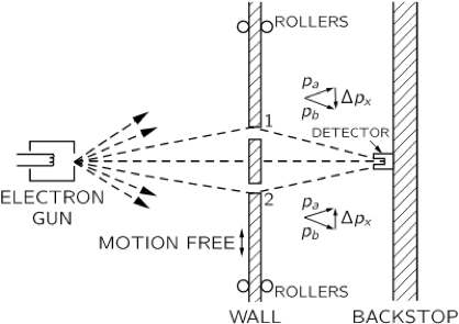
Let us
show for one particular case that the kind of relation given by Heisenberg must
be true in order to keep from getting into trouble. We imagine a modification
of the experiment of Fig. 1–3, in which the wall with
the holes consists of a plate mounted on rollers so that it can move freely up
and down (in the x-direction),
as shown in Fig. 1–6. By watching the motion of
the plate carefully we can try to tell which hole an electron goes through.
Imagine what happens when the detector is placed at x=0. We would expect that an
electron which passes through hole 1 must be deflected downward by the plate to
reach the detector. Since the vertical component of the electron momentum is
changed, the plate must recoil with an equal momentum in the opposite
direction. The plate will get an upward kick. If the electron goes through the
lower hole, the plate should feel a downward kick. It is clear that for every
position of the detector, the momentum received by the plate will have a
different value for a traversal via hole 1 than for a traversal via hole 2. So! Without disturbing
the electrons at all, but just by watching
the plate, we can tell which path the electron used.
Fig. 1–6. An experiment in which the recoil of the wall is measured.
Now in
order to do this it is necessary to know what the momentum of the screen is,
before the electron goes through. So when we measure the momentum after the
electron goes by, we can figure out how much the plate’s momentum has changed.
But remember, according to the uncertainty principle we cannot at the same time
know the position of the plate with an arbitrary accuracy. But if we do not
know exactly where the plate is, we cannot
say precisely where the two holes are. They will be in a different place for
every electron that goes through. This means that the center of our interference
pattern will have a different location for each electron. The wiggles of the
interference pattern will be smeared out. We shall show quantitatively in the
next chapter that if we determine the momentum of the plate sufficiently
accurately to determine from the recoil measurement which hole was used, then
the uncertainty in the x-position of the plate will, according to the
uncertainty principle, be enough to shift the pattern observed at the detector
up and down in the x-direction
about the distance from a maximum to its nearest minimum. Such a random shift
is just enough to smear out the pattern so that no interference is observed.
The
uncertainty principle “protects” quantum mechanics. Heisenberg recognized that
if it were possible to measure the momentum and the position simultaneously
with a greater accuracy, the quantum mechanics would collapse. So he proposed
that it must be impossible. Then people sat down and tried to figure out ways
of doing it, and nobody could figure out a way to measure the position and the
momentum of anything—a screen, an electron, a billiard ball, anything—with any
greater accuracy. Quantum mechanics maintains its perilous but still correct
existence.
NOTE: There is going to be no recoil up or down since electrons do not exist as lumps in space. They are a continuum of constant density. Heisenberg uncertainty principle only supports the concept of continuum; it does not account for varying density of the continuum. Here we have considerable scope for improving the mathematics of quantum mechanics.
Matter is substance and so is light (see The Logic of Substance). A substance has substantiality. The measure of substantiality is given by mass concentration. We may use the word “substantiality” to mean mass concentration.
By substantiality we mean mass concentration.
As shown in the chapter on The Logic of Field, the range of substantiality (mass concentration) was extended greatly with the discovery of the nuclear and electronic regions in the atom. The substantiality of nucleus is greater than the substantiality of matter. The substantiality of electron, on the other hand, is many orders of magnitude less than the substantiality of matter.
We apply the term “mass” to matter, but when we consider particles like protons, neutrons and electrons, we assume the mass to be distributed throughout the volume of the particle. Hence, we are dealing with mass concentration, or substantiality, at a location in space. We may, therefore, conclude:
A location in space has substantiality.
.
Substantiality and Energy
Einstein’s famous
equation, E = mc2 shows the equivalence of mass and energy. It
also shows that infinitesimal amount of mass is equivalent to a significant
amount of energy because of the large multiplier c2.
Therefore, an infinitesimal amount of mass may only be detectable as energy.
The mass of the electron field may be back calculated as E/c2, but it is so small a number that physics uses the equivalent energy value. to represent the substantiality of the electron field.
The presentation of substantiality
of field in energy units has, unfortunately, contributed to conflating the
traditional concepts of mass and energy. The energy units do not imply that
field has no substance.
The substantiality is expressed in mass units, but, for fields, it may be expressed in energy units.
.
Intrinsic Motion
The agitation of gas molecules is an example of intrinsic motion. Another example is the Brownian motion. These particles move by themselves. There are no external forces acting on these particles. Another example of intrinsic motion is the rapid motion of electron field around the nucleus.
The intrinsic motion of
a substance exists because of its intrinsic nature. Therefore, the intrinsic
motion must depend on substantiality. We may say that the rapid motion of
electron field around the nucleus exists because of the large substantiality
differential between these two regions within the atom.
The intrinsic motion of light expresses itself as the speed of light. Therefore, the speed of light is also an expression of the substantiality of light.
Substance has intrinsic motion that depends on substantiality.
.
Speed & Mass Concentration
The more substantial is the substance the greater is its endurance, the longer it stays in a state, and the slower is its rate of intrinsic change. This is the case with solid matter. On the other hand, the less substantial is the substance, the lesser is its endurance, the shorter it stays in a state, and the faster is its rate of intrinsic change. The is the case with ephemeral light. Therefore
The rate of intrinsic change is inversely proportional to substantiality.
The rate of intrinsic change for light appears to be its motion in space. This motion is absolute because it does not depend on anything external to light for its existence or specific nature. From this perspective, the absolute motion of matter is close to zero because its rate of intrinsic change in space is extremely slow. Therefore
The rate of intrinsic change appears as absolute motion in space.
The absolute motion is very different from relative motions of objects. The speed of light is 3 x 10⁸ meters/sec. This is a measure of absolute motion. The orbital speed of earth around the sun is about 3 x 10⁴ meters/sec. This is a measure of relative motion. We cannot say that the speed of earth is 1/10,000 of the speed of light because this is not comparing the same type of motion. The absolute motion of earth is very likely even a smaller percentage of the speed of light.
We cannot compare relative speeds to the speed of light.
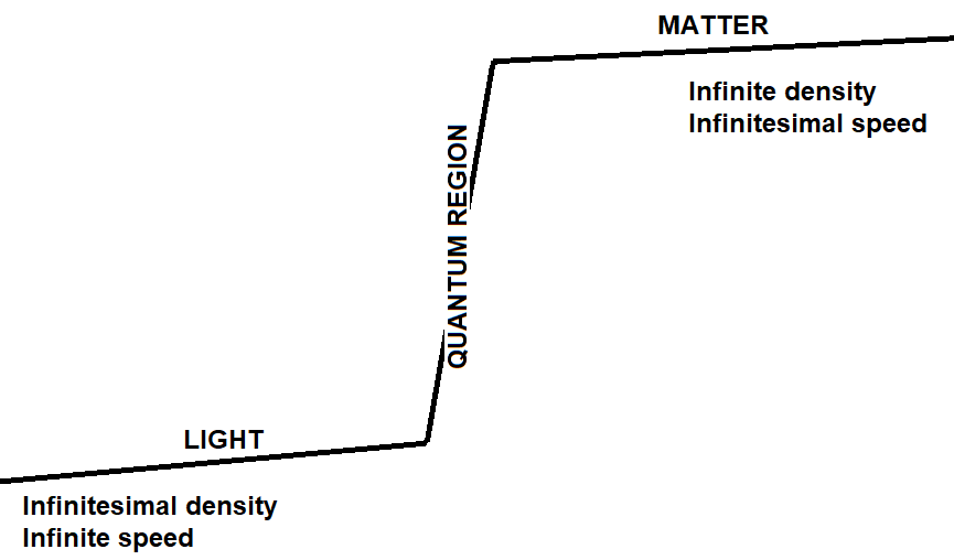
The speeds of material bodies and fields may only be compared in terms of their substantiality (mass concentration). This comparison is anticipated by the mass-energy equivalence. As the intrinsic mass is replaced by an equivalent amount of intrinsic energy, it has the effect of increasing the intrinsic motion of the substance. This may be demonstrated by the following sketch.
This leads to the conclusion that,
The intrinsic speed of substance is inversely proportional to its mass concentration.
The substantiality of
electromagnetic field (EMF) is much less than the substantiality of the
electronic region in the atom. Therefore, the EM field moves much more rapidly compared
to the electron field.
.
Additional Conclusions
We may expect a material body to be fixed in its natural velocity in space. If it is forced to accelerate by the application of external force, it will return to its natural velocity when that force is removed. It will not continue to move at its accelerated velocity forever. This conclusion modifies what Newton proposed.
If a material object is
continually accelerated by the application of a constant force (as in a
gravitational field), then its substantiality decreases with acceleration. This
change, however, may be imperceptible because of energy to mass ratio is c2to 1.
Any substance at
absolute rest must have infinite substantiality. Therefore, the substantiality
of postulated stationary aether shall be infinite. We do not experience space
being filled with a substance of infinite substantiality. Therefore, Einstein
was correct in discarding the notion of stationary aether.
The substantiality of
the EM field may be approximated by its frequency. Higher frequency would mean
higher substantiality. We may, therefore, expect the velocity of the field
substance to slightly decrease with increasing frequency.
The velocity of light is
generally measured at the frequency of visible light. We assume on the basis of
Maxwell’s theory that this velocity is the same throughout the EM spectrum. Maxwell’s
theory assumes an aether of uniform substantiality as the medium throughout the
EM spectrum. That may not be so.
The gravitational field
is expected to have a substantiality much less than that of the EM Field.
Therefore, the velocity of the gravitational field is expected to be higher
than the velocity of light
Implications of the
above on the special theory of relativity shall be covered later.
As shown in the paper, Physics & Reality, the logic of reality depends on its consistency. A strange shift in reality occurred when Newton’s corpuscular theory of light was replaced by the wave theory of light. Light was no longer viewed as substance; instead it was viewed as energy that propagated through a hypothetical medium (substance) called aether.
The reality in physics shifted from “light is substance” to “light is energy”.
NOTE: A substance is anything that has impact on senses. That impact is sensed as force.
.
Young’s Interference Experiment
The wave theory of light was at first resisted because there was no medium in which a light wave could travel. But Newton’s corpuscular theory could not explain the overwhelming evidence of the wave characteristics of light.
Young’s interference experiment, also called Young’s double-slit interferometer, was the original version of the modern double-slit experiment, performed at the beginning of the nineteenth century by Thomas Young. This experiment played a major role in the general acceptance of the wave theory of light.
With the acceptance of wave theory, physics was forced to postulate a hypothetical stationary aether.
The demonstration of interference patterns of light led to the acceptance of wave theory over Newton’s corpuscular theory.
.
Particles versus Wave
The corpuscles of Newton’s theory were discrete; therefore, they could not be modeled into waves to explain the interference patterns. But a closer look tells us that these corpuscles cannot be discrete.
Material particles are discrete by the fact of their center of mass. Light particles do not have center of mass, and, therefore, they cannot be distinguished from each other. They must form a fluid-like continuum of substance that flows. Newton’s corpuscular theory incorrectly visualized light to be made up of discrete particles.
When corpuscles are modeled as a flowing, fluid substance, the objections to corpuscular theory go away. Light becomes capable of explaining the interference patterns of Young’s experiment, without requiring a medium.
When corpuscles are seen as fluid-like flowing substance, they are able to explain Young’s interference patterns.
.
Quantum Reality and Mathematics
This shift of light as energy has persisted through Maxwell’s theory, Einstein theory of relativity, Quantum mechanics and now QED (Quantum electrodynamics) even when the hypothetical aether has long been discarded. The illusion of light as energy has been kept alive by the accuracy of results from these mathematical theories.
In his book, QED, The Strange Theory of Light and Matter, Richard Feynman takes up the difficult problem of partial reflection from glass surfaces. It has no satisfactory solution for light either as a discrete particle or as a continuous wave. So, QED has no choice but to resort to mathematical probability to explain the “strangeness of nature”.
But if we define light as a non-atomic fluid that has very low mass density and very high speed, the problem of partial reflection is resolved easily without thinking of the strangeness of nature. With this classical model one does not have to resort to mathematical probability to find a real answer.
Strangeness of reality comes from conflating energy with substance.
.
Future Possibility
The mathematical models of quantum physics have been successful in predicting physical phenomena in a certain narrow sense. It may be possible to reinterpret the mathematical symbolism of quantum physics without affecting those results.
By considering light to be a fluid-like, flowing, non-atomic substance we restore the consistency of reality. This consistency may spur just enough intuition to allow QED to successfully explain gravity and radioactivity as well.
The consistency in reality seems to spur intuition.